 RF cat corner
Graph nodes are states
Sep 16, 2026Introduction
When studying graph theory, the first examples proposed to students most often involve maps where nodes are geographical locations, edges physical roads with their distances, and path distances actual travel distances.
However, it is also possible to see nodes as states, as outlined in the following examples.
Example 1: routing problems with constraints
Inspired by a true problem.
Imagine a travel problem where travellers should calculate their trip so that they either go through country A, or through country B, or through neither, but must not go through both countries.
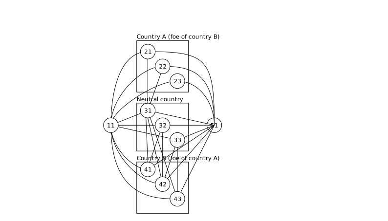
A possible solution to this problem would be to tweak the algorithm used to solve this graph: either calculating shortest routes between sub-domains, or calculating the k shortest routes to be able to take alternative paths in the case the shortest path is forbidden, and so on.
A more straightforward way is to consider states as nodes and to apply the usual algorithms directly. Here, the states would be like (11,none) for the starting node, (31,A) after (11,none)->(21,A), or (31,B) after (11,none)->(31,B), and so on. Note that this graph would be directional, which could surprise people used to the locations as nodes approach but is barely noticed for people used to the states as nodes approach.
The total number of nodes in this approach is multiplied by the number of the states. On the one hand, it can be troublesome for algorithms relying on various arrays to do their job, but this drawback may be overcome by the simplification of the algorithm. On the other hand, this is not at all a problem in cases the graph is stored in a sparse way or lazily evaluated.
Example 2: true states
While in the previous case the states can be seen as a convenient way to implement a constraint, in lots of cases the nodes are true states. A typical example is the study of a control flow inside a program. But there are more mundane cases.
I recently found this example in my drafts about a scheduling problem for the repair of various devices, the devices being able to be repaired only one at a time, and each device having a repair time and a cost per time unit. The example showed the application of Dijkstra’s algorithm.
| Device | Time | Unit Cost |
|---|---|---|
| Oven | 3 | 2 |
| Dishwasher (DiW) | 2 | 3 |
| Washing machine (WaM) | 5 | 4 |
| Computer (Comp) | 4 | 9 |
| Television (TV) | 6 | 5 |
Initial paths:
- (1): {Oven, DiW, WaM, Comp, TV} length 0.
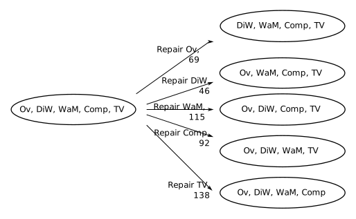
Step 1
Development of (1) of length 0.
Paths:
- (2): (1) -> {DiW, WaM, Comp, TV} length 69
- (3): (1) -> {Oven, WaM, Comp, TV} length 46
- (4): (1) -> {Oven, DiW, Comp, TV} length 115
- (5): (1) -> {Oven, WaM, DiW, TV} length 92
- (6): (1) -> {Oven, WaM, DiW, Comp} length 138
Shortest unvisited path: (3) length 46.
Step 2
Development of (3) length 46.
Paths:
- (7): (3) –60–> {WaM, Comp, TV} length 106
- (8): (3) –100–> {Oven, Comp, TV} length 146
- (9): (3) –80–> {Oven, WaM, TV} length 126
- (10): (3) –120–> {Oven, WaM, Comp} length 166
Shortest unvisited path: (2) length 69.
Step 3
Development of (2) length 69.
Paths:
- (11): (2) –42–> {WaM, Comp, TV} length 111
- (12): (2) –105–> {DiW, Comp, TV} length 174
- (13): (2) –84–> {DiW, WaM, TV} length 153
- (14): (2) –126–> {DiW, WaM, Comp} length 195
Shortest unvisited path: (5) length 92.
Steps 4 to 24
Removed for brevity, follow the same pattern.
Step 25
Development of (56) length 216.
Paths:
- (70): (56) –6–> {} length 222
Shortest unvisited path: (54) length 221.
Step 26
Development of (54) length 221.
Paths:
- (71): (54) –15–> {DiW} length 236
- (72): (54) –10–> {Oven} length 231
Shortest unvisited path: (70) length 222.
This path reaches the empty set (all devices repaired), ending the algorithm.
Conclusion
Path (70) reaches the empty set with a total cost of 222, corresponding to the repair order: Comp, DiW, TV, WaM, Oven. Since all remaining unvisited paths have a higher length, this is the optimal solution.
While a first approach to the analysis of a graph with constraints is to handle them with a locations as nodes approach and to use various techniques to process the constraints, handling them with a states as nodes approach can lead to simpler algorithms.