 RF cat corner
Equations for terminating a differential amplifier in single-ended input.
16 Jun 2025Introduction
A few years ago, I had to terminate a differential amplifier in single-ended input. Analog Devices AN-09901 gives equations for that. Unfortunately, there are an inaccuracy in these equations. According to this page, the input impedance for balanced differential input signals is given by
However, in this use case, the last equation is uncorrect. It would have been correct if the -DIN input were connected directly to ground. However, this is not the case, and instead this input is connected to ground through a resistor of value
Schematic
The schematic is shown below. Note the strange alignment of Rsp and Rsn. Rsp is part of the source while Rsn is part of the board. Note that in an actual implementation, Rsn and Rtn are likely to be merged. Details of the LTSpice simulation will be described at the end.

Calculation philosophy: solving vs. enforcing
There are two methods to calculate the values of the components in an electrical circuit:
-
Determine all the equations of all the wanted parameters (gain, impedance) in function of the components values, and invert all the equation. This is the solving approach.
-
Enforce at as soon as possible in the calculation process the wanted parameters by setting early some components values. This is the enforcing approach.
Calculations get much easier with the enforcing approach, in a similar approach than proposed by Middlebrook and its successors, notably Vorperian and Basso.
This case is a great illustration of this principle. I first tried the first approach, without success, thereafter the second approach, and got manageable equations.
Calculations details
Calculation of RG
It is assumed that RF is fixed. For current feedback amplifiers, common for high speed, RF contributes to the amplifier gain and have a value recommended by the datasheet which should be respected in most cases. For voltage feedback amplifiers having some speed, RF have to be low enough to avoid issues with the various parasitic capacitances which also leads to a recommended value.
Normalisation
After a long time working with these equations, I realized it was easier to use normalized values of the resistors, and the easiest value for normalization is the feedback resistor RF, as such:
Equation of &&V_X^+&&
Equation of &&V_X^-&&
Equations of &&V_X^+&& and &&V_X^-&& can be determined from Millman theorem2:
And their ratio can be calculated as such:
Using the previous expression of &&V_X^+&&, the actual value of &&V_X^-&& can be calculated as such:
Balance of &&V_"IN"^+&& and &&V_"IN"^-&&
In the normal operation of an operational amplifier, &&V_"IN"^+ = V_"IN"^-&&. Both quantities can be calculated as such, using again Millman theorem2:
And the condition &&V_"IN"^+ = V_"IN"^-&& can be written as such:
In which the values of &&V_X^+&& and &&V_X^-&& can be substituted:
Which can be put in a second order equation in the following way (note the early optimizations of the equations):
Solving the balance equation
This quadratic equation can be solved in the usual way3:
Usually, we say some things about the sign of &&\Delta&& and the existence of the roots. This will be left for a further release of this page. For now, just find the equations to put in Excel:
Leading to the final equation for &&R_G^’&&:
Calculation of &&R_T&&
For the calculation of &&R_T&&, the resistances are not normalized because the resulting expression is more meaningful.
&&R_T&& can be calculated by the usual way, a bit long. However, there is a quicker shortcut:
Impedance of &&R_G&&, &&R_F&&, and the amplifier can be calculated from the Miller formula4:
where the gain &&V_"OUT"/V_x^+&& can be calculated as such:
giving:
From this resistance, &&Z_"IN"&& can be calculated using the usual parallel resistor formula5:
which can be reversed as such:
leading to the final expression of &&R_T&&:
LTSpice simulation
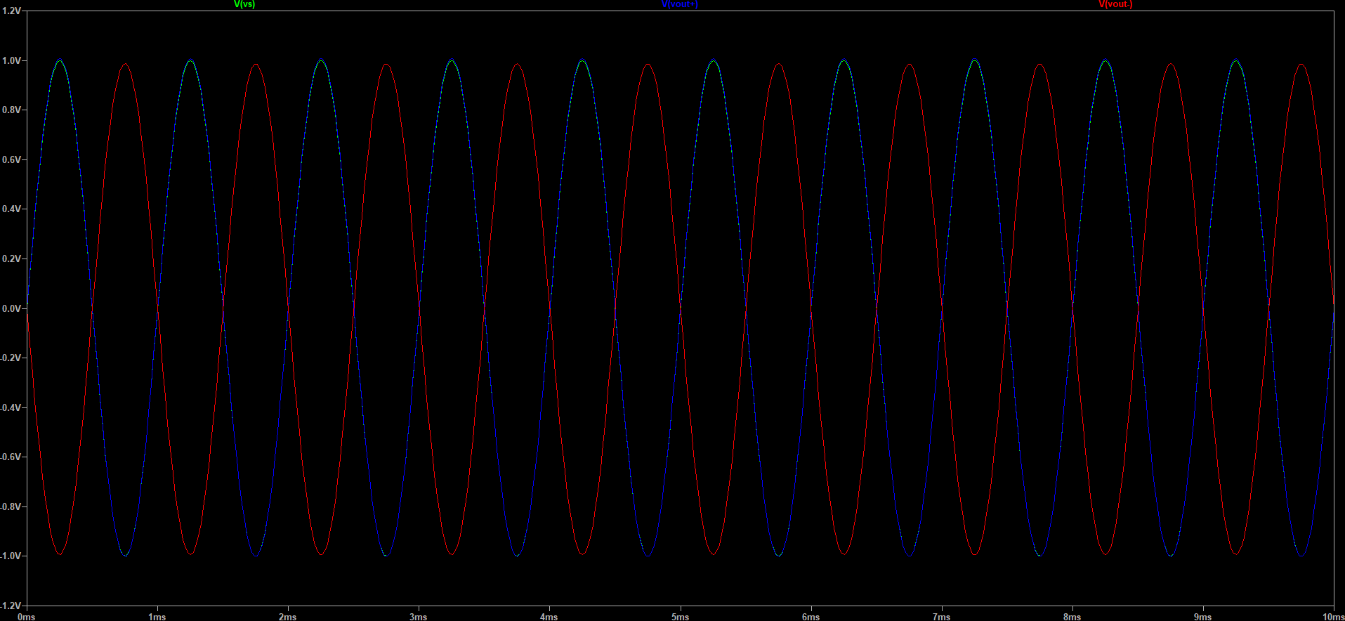
LTSpice simulation filed are provided here: diff-amp-SE-plot.asc and diff-amp-SE-plot.plt. Gain was set to 2 to allow easier check of proper operation by superimposing the curves.
Excel file
The Excel calculation file, self explanatory, can be downloaded here: diff-amp-SE-Excel.xlsx.