On stability of capacitive loaded op-amps, detailed equations.
19 Dec 2025
Isolation resistor + double feedback without RFx resistor
Before getting to the more complex case of the double feedback with RFx resistor, it is useful to study this case.
Operational amplifier output to feedback
V^- = (V_"AOP" \cdot C_F \cdot s + V_"out" / R_F) / (C_F \cdot s + 1 / R_F) = (V_"AOP" \cdot C_F \cdot s + V_"AOP" \cdot 1/(1+R_"iso" \cdot C_L \cdot s) \cdot 1 / R_F) / (C_F \cdot s + 1 / R_F)
V^- = V_"AOP" \cdot (C_F \cdot s + 1/(1+R_"iso" \cdot C_L \cdot s) \cdot 1 / R_F) / (C_F \cdot s + 1 / R_F)
V^- = V_"AOP" \cdot (R_F \cdot C_F \cdot s + 1/(1+R_"iso" \cdot C_L \cdot s)) / (R_F \cdot C_F \cdot s + 1)
Here the time constants can be introduced:
V^- = V_"AOP" \cdot (\tau_F \cdot s + 1/(1 + \tau_L \cdot s)) / (\tau_F \cdot s + 1)
V^- = V_"AOP" \cdot (1 + (\tau_F \cdot s) \cdot (1 + \tau_L \cdot s)) / ((1 + \tau_F \cdot s) \cdot (1 + \tau_L \cdot s))
V^- = V_"AOP" \cdot (1 + \tau_F \cdot s + \tau_F \cdot \tau_L \cdot s^2) / ((1 + \tau_F \cdot s) \cdot (1 + \tau_L \cdot s))
Closed loop AOP gain
V_"AOP" = (V_"in" - V^-) \cdot "GBW"/s
V_"AOP" = V_"in" \cdot "GBW"/s - V^- \cdot "GBW"/s
V_"AOP" = V_"in" \cdot "GBW"/s - V_"AOP" \cdot
(1 + \tau_F \cdot s + \tau_F \cdot \tau_L \cdot s^2) / ((1 + \tau_F \cdot s) \cdot (1 + \tau_L \cdot s)) \cdot "GBW"/s
V_"AOP" \cdot [ 1 + (1 + \tau_F \cdot s + \tau_F \cdot \tau_L \cdot s^2) / ((1 + \tau_F \cdot s) \cdot (1 + \tau_L \cdot s)) \cdot "GBW"/s ]
= V_"in" \cdot "GBW" / s
V_"AOP" \cdot [ 1 + ("GBW" + "GBW" \cdot \tau_F \cdot s + "GBW" \cdot \tau_F \cdot \tau_L \cdot s^2) / ((1 + \tau_F \cdot s) \cdot (1 + \tau_L \cdot s) \cdot s) ]
= V_"in" \cdot "GBW" / s
V_"AOP" \cdot ( (s + (\tau_F + \tau_S) \cdot s^2 + \tau_F \cdot \tau_L \cdot s^3) + ("GBW" + "GBW" \cdot \tau_F \cdot s + "GBW" \cdot \tau_F \cdot \tau_L \cdot s^2) ) / ((1 + \tau_F \cdot s) \cdot (1 + \tau_L \cdot s) \cdot s)
= V_"in" \cdot "GBW" / s
V_"AOP" \cdot ( "GBW" + (1 + "GBW" \cdot \tau_F) \cdot s + (\tau_F + \tau_S + "GBW" \cdot \tau_F \cdot \tau_L) \cdot s^2 + \tau_F \cdot \tau_L \cdot s^3 ) / ((1 + \tau_F \cdot s) \cdot (1 + \tau_L \cdot s) \cdot s)
= V_"in" \cdot "GBW" / s
Factorizing by "GBW" and 1/s:
V_"AOP" \cdot ( 1 + (\tau_F + 1 / "GBW") \cdot s + (\tau_F \cdot \tau_L + (\tau_F + \tau_L) / "GBW") \cdot s^2 + (\tau_F \cdot \tau_L) / "GBW" \cdot s^3 ) / ((1 + \tau_F \cdot s) \cdot (1 + \tau_L \cdot s))
= V_"in"
Inverting:
V_"AOP"
= ((1 + \tau_F \cdot s) \cdot (1 + \tau_L \cdot s)) / ( 1 + (\tau_F + 1 / "GBW") \cdot s + (\tau_F \cdot \tau_L + (\tau_F + \tau_L) / "GBW") \cdot s^2 + (\tau_F \cdot \tau_L) / "GBW" \cdot s^3 ) \cdot V_"in"
Seek factorization on the form:
\begin{align}
& D(s) \\
& = (1 + 2 \cdot \zeta \cdot \tau_{p0} \cdot s + \tau_{p0}^2 \cdot s^2) \cdot (1 + \tau_{p1} \cdot s) \\
& = 1 + (2 \cdot \zeta \cdot \tau_{p0} + \tau_{p1}) \cdot s + (\tau_{p0}^2 + 2 \cdot \zeta \cdot \tau_{p0} \cdot \tau_{p1}) \cdot s^2 + \tau_{p0}^2 \cdot \tau_{p1} \cdot s^3
\end{align}
Leading to following equations:
\begin{align}
2 \cdot \zeta \cdot \tau_{p0} + \tau_{p1} &= \tau_F + \frac{1}{\text{GBW}} \\
\tau_{p0}^2 + 2 \cdot \zeta \cdot \tau_{p0} \cdot \tau_{p1} &= \tau_F \cdot \tau_L + \frac{\tau_F + \tau_L}{\text{GBW}} \\
\tau_{p0}^2 \cdot \tau_{p1} &= \frac{\tau_F \cdot \tau_L}{\text{GBW}}
\end{align}
Approximating using: \tau_{p0}^2 \gg 2 \cdot \zeta \cdot \tau_{p0} \cdot \tau_{p1}:
\begin{align}
\tau_{p0}^2 &\approx \tau_F \cdot \tau_L + \frac{\tau_F + \tau_L}{\text{GBW}} \\
\left[ \tau_F \cdot \tau_L + \frac{\tau_F + \tau_L}{\text{GBW}} \right] \cdot \tau_{p1} &\approx \frac{\tau_F \cdot \tau_L}{\text{GBW}} \\
2 \cdot \zeta \cdot \tau_{p0} + \tau_{p1} &= \tau_F + \frac{1}{\text{GBW}}
\end{align}
Equation of last pole:
\begin{align}
\left[ \text{GBW} + \frac{\tau_F + \tau_L}{\tau_F \cdot \tau_L} \right] \cdot \tau_{p1} \approx 1 \\
\left[ \text{GBW} + \frac{1}{\tau_F} + \frac{1}{\tau_L} \right] \cdot \tau_{p1} \approx 1 \\
\tau_{p1} \approx \frac{1}{\text{GBW} + \frac{1}{\tau_F} + \frac{1}{\tau_L}}
\end{align}
AOP dominant. Equation of damping:
\begin{align}
2 \cdot \zeta \cdot \tau_{p0} + \tau_{p1} &= \tau_F + \frac{1}{\text{GBW}} \\
\zeta &\approx \frac
{ \tau_F + \frac{1}{\text{GBW}} - \frac{1}{\text{GBW} + \frac{1}{\tau_F} + \frac{1}{\tau_L}} }
{ 2 \cdot \sqrt{\tau_F \cdot \tau_L + \frac{\tau_F + \tau_L}{\text{GBW}}} }
\end{align}
The upper term can be simplified as such:
\begin{align}
& \frac{1}{\text{GBW}} - \frac{1}{\text{GBW} + \frac{1}{\tau_F} + \frac{1}{\tau_L}} \\
& = \frac
{\text{GBW} + \frac{1}{\tau_F} + \frac{1}{\tau_L} - \text{GBW}}
{\text{GBW} \cdot \left( \text{GBW} + \frac{1}{\tau_F} + \frac{1}{\tau_L} \right)} \\
& = \frac
{ \frac{1}{\tau_F} + \frac{1}{\tau_L} }
{\text{GBW} \cdot \left( \text{GBW} + \frac{1}{\tau_F} + \frac{1}{\tau_L} \right)} \\
& = \frac
{ \tau_F + \tau_L }
{\text{GBW} \cdot \left( \text{GBW} \cdot \tau_F \cdot \tau_L + \tau_F + \tau_L \right)}
\end{align}
Giving:
\begin{align}
\zeta &\approx \frac
{
\tau_F
+ \frac
{ \tau_F + \tau_L }
{\text{GBW} \cdot \left( \text{GBW} \cdot \tau_F \cdot \tau_L + \tau_F + \tau_L \right)}
}
{ 2 \cdot \sqrt{\tau_F \cdot \tau_L + \frac{\tau_F + \tau_L}{\text{GBW}}} }
\end{align}
The value for "GBW" = \infty can be outlined as such:
\begin{align}
\zeta &\approx
\frac
{ \tau_F }
{
2 \cdot \sqrt{\tau_F \cdot \tau_L}
} \cdot
\frac
{
1
+ \frac
{ \tau_F + \tau_L }
{\text{GBW} \cdot \tau_F \cdot \left( \text{GBW} \cdot \tau_F \cdot \tau_L + \tau_F + \tau_L \right)}
}
{ \sqrt{ 1 + \frac{\tau_F + \tau_L}{\text{GBW} \cdot \tau_F \cdot \tau_L} } } \\
&\approx
\sqrt{
\frac
{ \tau_F }
{ 4 \cdot \tau_L }
} \cdot
\frac
{
1
+ \frac
{ \tau_F + \tau_L }
{\text{GBW} \cdot \tau_F \cdot \left( \text{GBW} \cdot \tau_F \cdot \tau_L + \tau_F + \tau_L \right)}
}
{ \sqrt{ 1 + \frac{\tau_F + \tau_L}{\text{GBW} \cdot \tau_F \cdot \tau_L} } }
\end{align}
This last expression shows that to have an aperiodic answer, the time constant of the feedback network must be at least 4 times the time constant of the output RC. In this case, the feedback network ensures DC accuracy and stability, but for higher frequencies, this scheme is equivalent to a simple voltage followed followed by the RC network, without any improvement on its bandwidth, which lead to the desire of feedback schemes who provide actual bandwidth improvement.
Isolation resistor + double feedback with RFx resistor
Operational amplifier output to feedback
V^- = (V_"AOP" / (R_(Fx) + 1 / (C_F \cdot s)) + V_"out" / R_F) / (1 / (R_(Fx) + 1 / (C_F \cdot s)) + 1 / R_F) = (V_"AOP" / (R_(Fx) + 1 / (C_F \cdot s)) + V_"AOP" \cdot 1/(1+R_"iso" \cdot C_L \cdot s) \cdot 1 / R_F) / (1 / (R_(Fx) + 1 / (C_F \cdot s)) + 1 / R_F)
V^- = V_"AOP" \cdot (1 / (R_(Fx) + 1 / (C_F \cdot s)) + 1/(1+R_"iso" \cdot C_L \cdot s) \cdot 1 / R_F) / (1 / (R_(Fx) + 1 / (C_F \cdot s)) + 1 / R_F)
V^- = V_"AOP" \cdot (R_F / (R_(Fx) + 1 / (C_F \cdot s)) + 1/(1+R_"iso" \cdot C_L \cdot s)) / (R_F / (R_(Fx) + 1 / (C_F \cdot s)) + 1)
V^- = V_"AOP" \cdot ( R_F / (R_(Fx) + 1 / (C_F \cdot s)) \cdot (1+R_"iso" \cdot C_L \cdot s) + 1 ) / ( (R_F / (R_(Fx) + 1 / (C_F \cdot s)) + 1) \cdot (1+R_"iso" \cdot C_L \cdot s) )
V^- = ( V_"AOP" \cdot R_F \cdot (1+R_"iso" \cdot C_L \cdot s) + R_(Fx) + 1 / (C_F \cdot s) ) / ( (R_F + R_(Fx) + 1 / (C_F \cdot s)) \cdot (1+R_"iso" \cdot C_L \cdot s) )
V^- = V_"AOP" \cdot ( R_F \cdot (1+R_"iso" \cdot C_L \cdot s) \cdot C_F \cdot s + R_(Fx) \cdot C_F \cdot s + 1 ) / ( [ 1 + (R_F + R_(Fx)) \cdot C_F \cdot s ] \cdot (1+R_"iso" \cdot C_L \cdot s) )
V^- = V_"AOP" \cdot ( R_F \cdot C_F \cdot s + R_"iso" \cdot C_L \cdot R_F \cdot C_F \cdot s^2 + R_(Fx) \cdot C_F \cdot s + 1 ) / ( [ 1 + (R_F + R_(Fx)) \cdot C_F \cdot s ] \cdot (1+R_"iso" \cdot C_L \cdot s) )
V^- = V_"AOP" \cdot ( R_F \cdot C_F \cdot s + R_"iso" \cdot C_L \cdot R_F \cdot C_F \cdot s^2 + R_(Fx) \cdot C_F \cdot s + 1 ) / ( (1+R_"iso" \cdot C_L \cdot s) \cdot [ 1 + (R_F + R_(Fx)) \cdot C_F \cdot s ] )
V^- = V_"AOP" \cdot ( 1 + ( R_F + R_(Fx) ) \cdot C_F \cdot s + R_"iso" \cdot C_L \cdot R_F \cdot C_F \cdot s^2 ) / ( (1+R_"iso" \cdot C_L \cdot s) \cdot [ 1 + (R_F + R_(Fx)) \cdot C_F \cdot s ] )
To avoid overshoots in the transfer function, it is seeked that the numerator has real roots, corresponding to time constants named conveniently \tau_3 and \tau_4, sorted in such a way that \tau_3 >= \tau_4. The denominator has two real roots, corresponding to the time constant R_"iso"\cdot C_L and to a time constant \tau_2=(R_F+R_(Fx)) \cdot C_F. Viete’s relations show that \tau_3+\tau_4=1+(R_F+R_(Fx)) \cdot C_F and hence that \tau_3+\tau_4=\tau_2. Thus, these constants can be ordered and renamed as follows:
\tau_2 >= \tau_3 >= \tau_4
For stability reasons, the phase shift at the unity gain frequency must be low enough because the op-amp has already a 90° phase shift, so \tau_4 >= \tau_"min", with \tau_"min" sufficiently lower than the time constant of the unity gain frequency.
Closed loop AOP gain
V_"AOP" = (V_"in" - V_x) \cdot "GBW"/s
V_"AOP" = V_"in" \cdot "GBW"/s - V_x \cdot "GBW"/s
V_"AOP" = V_"in" \cdot "GBW"/s - V_"AOP" \cdot
( 1 + (R_F + R_(Fx)) \cdot C_F \cdot s + R_"iso" \cdot R_F \cdot C_L \cdot C_F \cdot s^2 ) /
(1 + (R_"iso" \cdot C_L + (R_F + R_(Fx)) \cdot C_F) \cdot s + R_"iso" \cdot (R_F + R_(Fx)) \cdot C_L \cdot C_F \cdot s^2 ) \cdot "GBW"/s
V_"AOP" \cdot [ 1 + ( 1 + (R_F + R_(Fx)) \cdot C_F \cdot s + R_"iso" \cdot R_F \cdot C_L \cdot C_F \cdot s^2 ) /
(1 + (R_"iso" \cdot C_L + (R_F + R_(Fx)) \cdot C_F) \cdot s + R_"iso" \cdot (R_F + R_(Fx)) \cdot C_L \cdot C_F \cdot s^2 ) \cdot "GBW"/s ]
= V_"in" \cdot "GBW" / s
V_"AOP" \cdot [ 1 + ( "GBW" + "GBW" \cdot (R_F + R_(Fx)) \cdot C_F \cdot s + "GBW" \cdot R_"iso" \cdot R_F \cdot C_L \cdot C_F \cdot s^2 ) /
(s + (R_"iso" \cdot C_L + (R_F + R_(Fx)) \cdot C_F) \cdot s^2 + R_"iso" \cdot (R_F + R_(Fx)) \cdot C_L \cdot C_F \cdot s^3 ) ]
= V_"in" \cdot "GBW" / s
V_"AOP" \cdot
( "GBW" + [1 + "GBW" \cdot (R_F + R_(Fx)) \cdot C_F] \cdot s + (R_"iso" \cdot C_L + (R_F + R_(Fx)) \cdot C_F + "GBW" \cdot R_"iso" \cdot R_F \cdot C_L \cdot C_F) \cdot s^2 + R_"iso" \cdot (R_F + R_(Fx)) \cdot C_L \cdot C_F \cdot s^3 ) /
( s + (R_"iso" \cdot C_L + (R_F + R_(Fx)) \cdot C_F) \cdot s^2 + R_"iso" \cdot (R_F + R_(Fx)) \cdot C_L \cdot C_F \cdot s^3 )
= V_"in" \cdot "GBW" / s
V_"AOP" = V_"in" \cdot "GBW" / s \cdot
( s + (R_"iso" \cdot C_L + (R_F + R_(Fx)) \cdot C_F) \cdot s^2 + R_"iso" \cdot (R_F + R_(Fx)) \cdot C_L \cdot C_F \cdot s^3 ) /
( "GBW" + [1 + "GBW" \cdot (R_F + R_(Fx)) \cdot C_F] \cdot s + (R_"iso" \cdot C_L + (R_F + R_(Fx)) \cdot C_F + "GBW" \cdot R_"iso" \cdot R_F \cdot C_L \cdot C_F) \cdot s^2 + R_"iso" \cdot (R_F + R_(Fx)) \cdot C_L \cdot C_F \cdot s^3 )
V_"AOP" = V_"in" \cdot
( 1 + (R_"iso" \cdot C_L + (R_F + R_(Fx)) \cdot C_F) \cdot s + R_"iso" \cdot (R_F + R_(Fx)) \cdot C_L \cdot C_F \cdot s^2 ) /
( 1 + [1 / "GBW" + (R_F + R_(Fx)) \cdot C_F] \cdot s + ((R_"iso" \cdot C_L + (R_F + R_(Fx)) \cdot C_F) / "GBW" + R_"iso" \cdot R_F \cdot C_L \cdot C_F) \cdot s^2 + (R_"iso" \cdot (R_F + R_(Fx)) \cdot C_L \cdot C_F) / "GBW" \cdot s^3 )
Output at the capacitive load
V_"out" = V_"AOP" \cdot (1/(C_L \cdot s))/(R_"iso"+1/(C_L \cdot s)) = V_"AOP" \cdot 1/(1+R_"iso" \cdot C_L \cdot s)
V_"out" = V_"in" \cdot
( 1 + (R_"iso" \cdot C_L + (R_F + R_(Fx)) \cdot C_F) \cdot s + R_"iso" \cdot (R_F + R_(Fx)) \cdot C_L \cdot C_F \cdot s^2 ) /
( 1 + [1 / "GBW" + (R_F + R_(Fx)) \cdot C_F] \cdot s + ((R_"iso" \cdot C_L + (R_F + R_(Fx)) \cdot C_F) / "GBW" + R_"iso" \cdot R_F \cdot C_L \cdot C_F) \cdot s^2 + (R_"iso" \cdot (R_F + R_(Fx)) \cdot C_L \cdot C_F) / "GBW" \cdot s^3 )
\cdot 1/(1+R_"iso" \cdot C_L \cdot s)
The numerator can be factored as such:
N(s) = [1 + R_"iso" \cdot C_L \cdot s] \cdot [1 + (R_F + R_(Fx)) \cdot C_F \cdot s]
Leading to a simpler expression:
V_"out" = V_"in" \cdot
[1 + (R_F + R_(Fx)) \cdot C_F \cdot s] /
( 1 + [1 / "GBW" + (R_F + R_(Fx)) \cdot C_F] \cdot s + ((R_"iso" \cdot C_L + (R_F + R_(Fx)) \cdot C_F) / "GBW" + R_"iso" \cdot R_F \cdot C_L \cdot C_F) \cdot s^2 + (R_"iso" \cdot (R_F + R_(Fx)) \cdot C_L \cdot C_F) / "GBW" \cdot s^3 )
The only practical way to handle this is to assume a big enough GBW:
V_"out" = V_"in" \cdot
[1 + (R_F + R_(Fx)) \cdot C_F \cdot s] /
( 1 + (R_F + R_(Fx)) \cdot C_F \cdot s + R_"iso" \cdot R_F \cdot C_L \cdot C_F \cdot s^2 )
Poles and zeros of the closed loop transfer function
This transfer function has the time constants previously found: a zero with time constant \tau_2=(R_F+R_(Fx)) \cdot C_F and two poles with times constants \tau_3 and \tau_4 such as \tau_3+\tau_4=\tau_2.
For the transfert function to be as close as possible to an ideal single-pole function, the zero time constant \tau_2 should be close enough to one of the time constants of the poles, \tau_3 or \tau_4.
Since \tau_3+\tau_4=\tau_2 and \tau_3>=\tau_4, this lead to \tau_2 \approx \tau_3 \gg \tau_4.
Loop gain, stability, and omega max
The loop gain is:
L = \frac{\text{GBW}}{s} \cdot
\frac{
1 + \left( R_F + R_{Fx} \right) \cdot C_F \cdot s + R_\text{iso} \cdot C_L \cdot R_F \cdot C_F \cdot s^2
}{
\left( 1 + R_\text{iso} \cdot C_L \cdot s \right) \cdot \left[ 1 + (R_F + R_{Fx}) \cdot C_F \cdot s \right]
}
Plugging into this equation the time constants:
L = \text{GBW} \cdot
\frac{
(1 + \tau_3 \cdot s) \cdot (1 + \tau_4 \cdot s)
}{
\left( 1 + \tau_L \cdot s \right) \cdot \left( 1 + \tau_2 \cdot s \right) \cdot s
}
Using the relations between time constants:
L = \text{GBW} \cdot
\frac{
(1 + \tau_3 \cdot s) \cdot (1 + \tau_4 \cdot s)
}{
\left( 1 + \tau_L \cdot s \right) \cdot \left[ 1 + \left( \tau_3 + \tau_4 \right) \cdot s \right] \cdot s
}
At the unity gain frequency to be calculated:
\begin{align*}
\left| L(\omega_0) \right| &= \left| \text{GBW} \cdot
\frac{
(1 + j \cdot \tau_3 \cdot \omega_0) \cdot (1 + j \cdot \tau_4 \cdot \omega_0)
}{
\left( 1 + j \cdot \tau_L \cdot \omega_0 \right) \cdot \left[ 1 + j \cdot \left( \tau_3 + \tau_4 \right) \cdot \omega_0 \right] \cdot j \cdot \omega_0
} \right| \\
&= \text{GBW} \cdot
\frac{
\left| 1 + j \cdot \tau_3 \cdot \omega_0 \right| \cdot \left| 1 + j \cdot \tau_4 \cdot \omega_0 \right|
}{
\left| 1 + j \cdot \tau_L \cdot \omega_0 \right| \cdot \left| 1 + j \cdot \left( \tau_3 + \tau_4 \right) \cdot \omega_0 \right| \cdot \omega_0
}
\end{align*}
Since for stability reasons the unity gain frequency is much greater than the other poles and zeros, it can be simplified as such:
\begin{align*}
\left| L(\omega_0) \right| &= \text{GBW} \cdot
\frac{
\tau_3 \cdot \omega_0 \cdot \tau_4 \cdot \omega_0
}{
\tau_L \cdot \omega_0 \cdot \left( \tau_3 + \tau_4 \right) \cdot \omega_0 \cdot \omega_0
} \\
&= \text{GBW} \cdot
\frac{
\tau_3 \cdot \tau_4
}{
\tau_L \cdot \left( \tau_3 + \tau_4 \right)
} \cdot \frac{1}{\omega_0} \\
&= \text{GBW} \cdot
\frac{
1
}{
\tau_L \cdot \left( \frac{1}{\tau_3} + \frac{1}{\tau_4} \right)
} \cdot \frac{1}{\omega_0} \\
\end{align*}
Since \tau_4 depends on \omega_0 because it must be high enough compared to 1/\omega_0, it is useful to introduce a product k_4 = \tau_4 \cdot \omega_0. 5 can be used as a starting point for a convenient phase shift. With this:
\begin{align*}
\left| L(\omega_0) \right| &= \text{GBW} \cdot
\frac{
1
}{
\tau_L \cdot \left( \frac{1}{\tau_3} + \frac{\omega_0}{k_4} \right)
} \cdot \frac{1}{\omega_0} \\
\end{align*}
Solving this equation:
\begin{align*}
& \left| L(\omega_0) \right| = 1 \\
& \text{GBW} \cdot
\frac{
1
}{
\tau_L \cdot \left( \frac{1}{\tau_3} + \frac{\omega_0}{k_4} \right)
} \cdot \frac{1}{\omega_0} = 1 \\
& \text{GBW} = \tau_L \cdot \left( \frac{1}{\tau_3} + \frac{\omega_0}{k_4} \right) \cdot \omega_0 \\
\end{align*}
This equation will be solved in two ways: a zero order approximation to have a tendency, and a first order approximation based on this tendency.
Since \tau_3 \gg \tau_4, the equation can be simplified as such:
\begin{align*}
& \text{GBW} \approx \tau_L \cdot \frac{\omega_0}{k_4} \cdot \omega_0 = \frac{\tau_L \cdot \omega_0^2}{k_4} \\
& \omega_0 = \sqrt{\frac{\text{GBW} \cdot k_4}{\tau_L}}
\end{align*}
Components values for the unit loop gain
Taking again the expression for the loop gain:
\begin{align*}
\left| L(\omega_0) \right| &= \text{GBW} \cdot
\frac{
\tau_3 \cdot \tau_4
}{
\tau_L \cdot \left( \tau_3 + \tau_4 \right)
} \cdot \frac{1}{\omega_0} \\
\end{align*}
Plugging inside the relations between \tau_3 \cdot \tau_4, \tau_3+\tau_4, \tau_L and the component values:
\begin{align*}
\left| L(\omega_0) \right| &= \frac{\text{GBW}}{\omega_0} \cdot
\frac{
R_\text{iso} \cdot C_L \cdot R_F \cdot C_F
}{
R_\text{iso} \cdot C_L \cdot \left( R_F + R_{Fx} \right) \cdot C_F
} \\
&= \frac{\text{GBW}}{\omega_0} \cdot \frac{R_F}{R_F + R_{Fx}} \\
\end{align*}
Since \left| L(\omega_0) \right| = 1:
\begin{align*}
\frac{R_F}{R_F + R_{Fx}} = \frac{\omega_0}{\text{GBW}} = \sqrt{\frac{k_4}{\text{GBW} \cdot \tau_L}} \\
\end{align*}
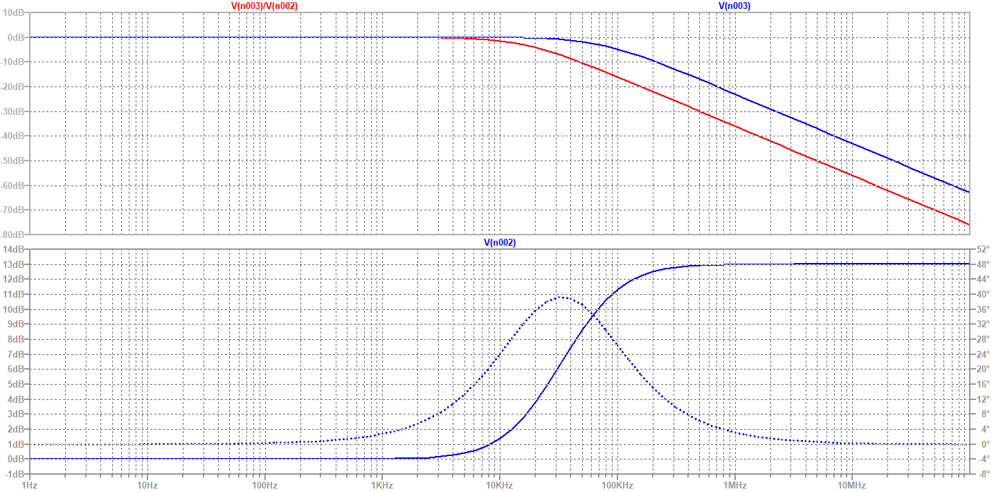
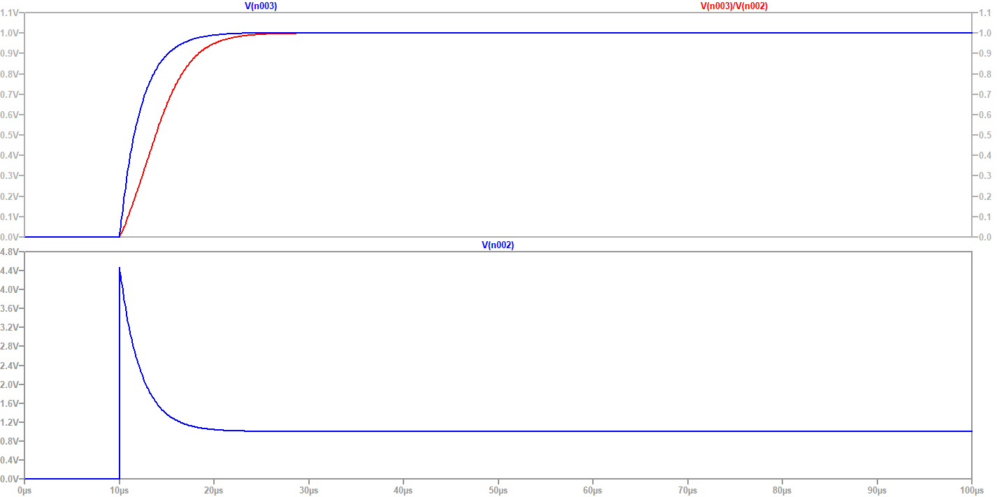
LTSpice simulation
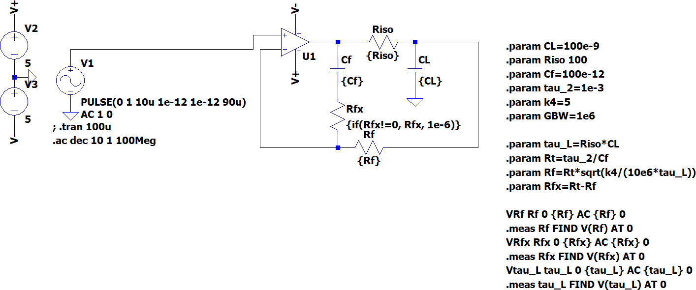
 RF cat corner