Simple calculations for active bandpass filter with finite GBW operational amplifier.

31 Dec 2025

Many thanks to Christophe Basso for his help in this work.

Introduction

Active filters are a convenient way to implement low frequency bandpass filters, and design equations are commonly available. However, their accuracy is often disappointing, with centre frequency often shifted, because they don't take into account the finite GBW (gain bandwidth product) of the operational amplifier used, particularly for common and low cost amplifiers with low GBW (gain bandwidth product) like the popular LM324. We propose here simple equations which take this into account and free and open source calculation tools.

Calculator

Simpler than the equations, you can directly jump on the following calculator which conveniently computes all the requested components values from the desired center frequency and bandwidth.

Input parameters

Center Frequency (f₀): Hz

Bandwidth (BW): Hz

Op-Amp GBW: Hz

Capacitor (C): F

Component values

In the current release, the gain is always set as its maximum. This will be fixed in a future release.

R₁: Ω

R₂: Ω

R₃: ∞ (Do not connect) ✅

Validity conditions

\frac{f_p}{\text{BW}} \geq 10

Transfer function plot

Equations for Excel spreadsheets

Synthesis equations

For people wanting or needing to implement these calculations in an Excel spreadsheet, here are the equations to be used. The usual equations to calculate the component values assuming an ideal operational amplifier with infinite GBW are:

\cases{ R_2 = \frac{1}{\pi \cdot \text{BW} \cdot C} \\ R_\text{TH} = \frac{\text{BW}}{4 \cdot \pi \cdot f_0^2 \cdot C} }

New equations taking info account the finite GBW are:

\cases{ R_2 = \left. \frac{1}{\pi \cdot \text{BW} \cdot C} \cdot \left[ 1 - \frac{\text{BW}}{\text{GBW}} \right] \middle/ \left[ 1 + \frac{2 f_0^2}{\text{BW} \cdot \text{GBW}} \right]\right. \\ R_\text{TH} = \frac{\text{BW}}{4 \cdot \pi \cdot f_0^2 \cdot C} }

Parasitic low-pass filter

A consequence of the finite GBW is the apparition of a parasitic low-pass filter with a cut-off frequency fp given by:

f_p = \left. \text{GBW} \cdot \left[ 1 + \frac{2 f_0^2}{\text{BW} \cdot \text{GBW}} \right] \middle/ \left[ 1 - \frac{\text{BW}}{\text{GBW}} \right] \right.

which is indeed slightly higher than GBW.

Validity conditions of the formulas

Once the parasitic pole is calculated, the validity conditions is the following:

\frac{f_p}{\text{BW}} \geq 10

Example with Excel spreadsheet

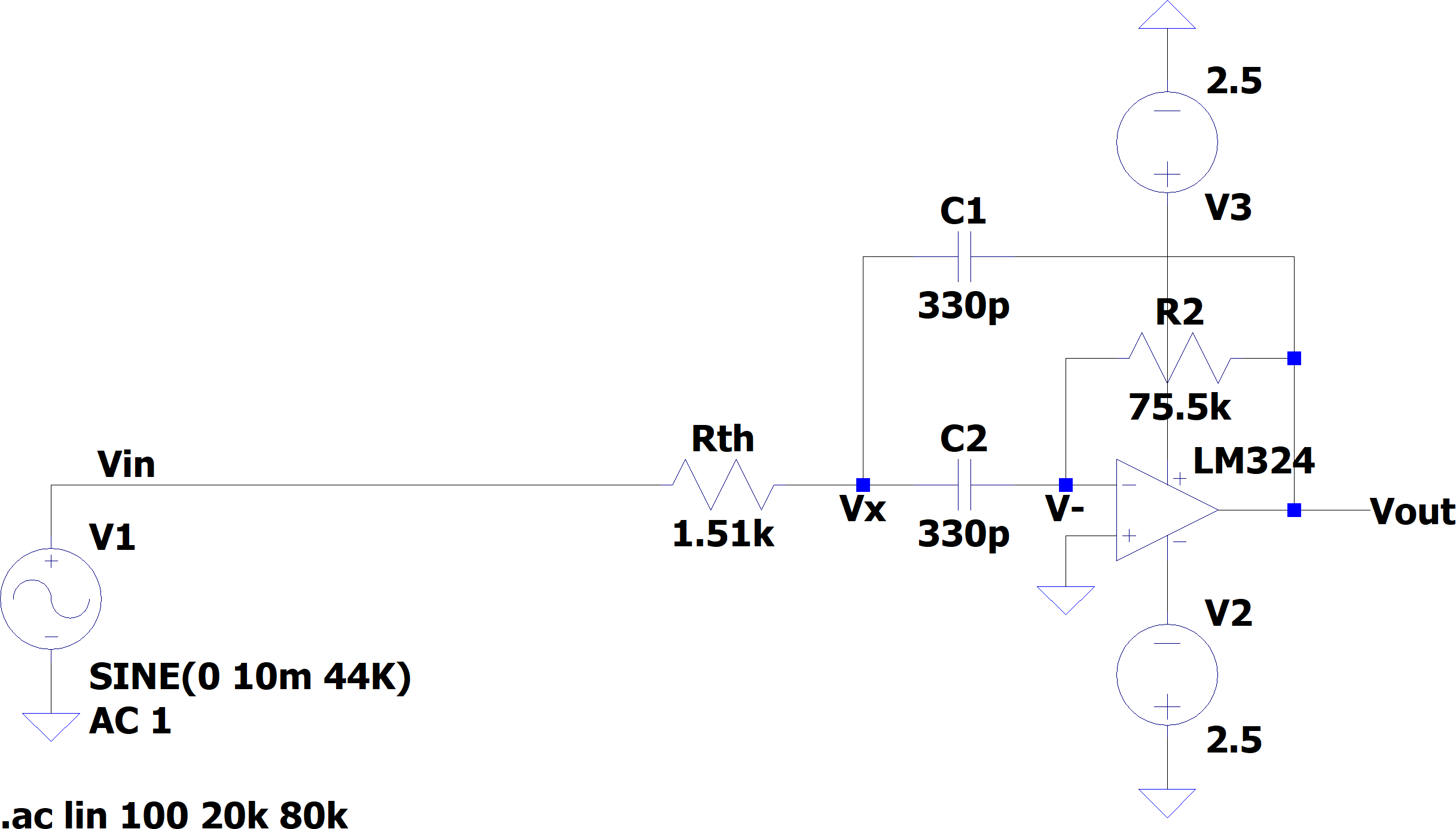
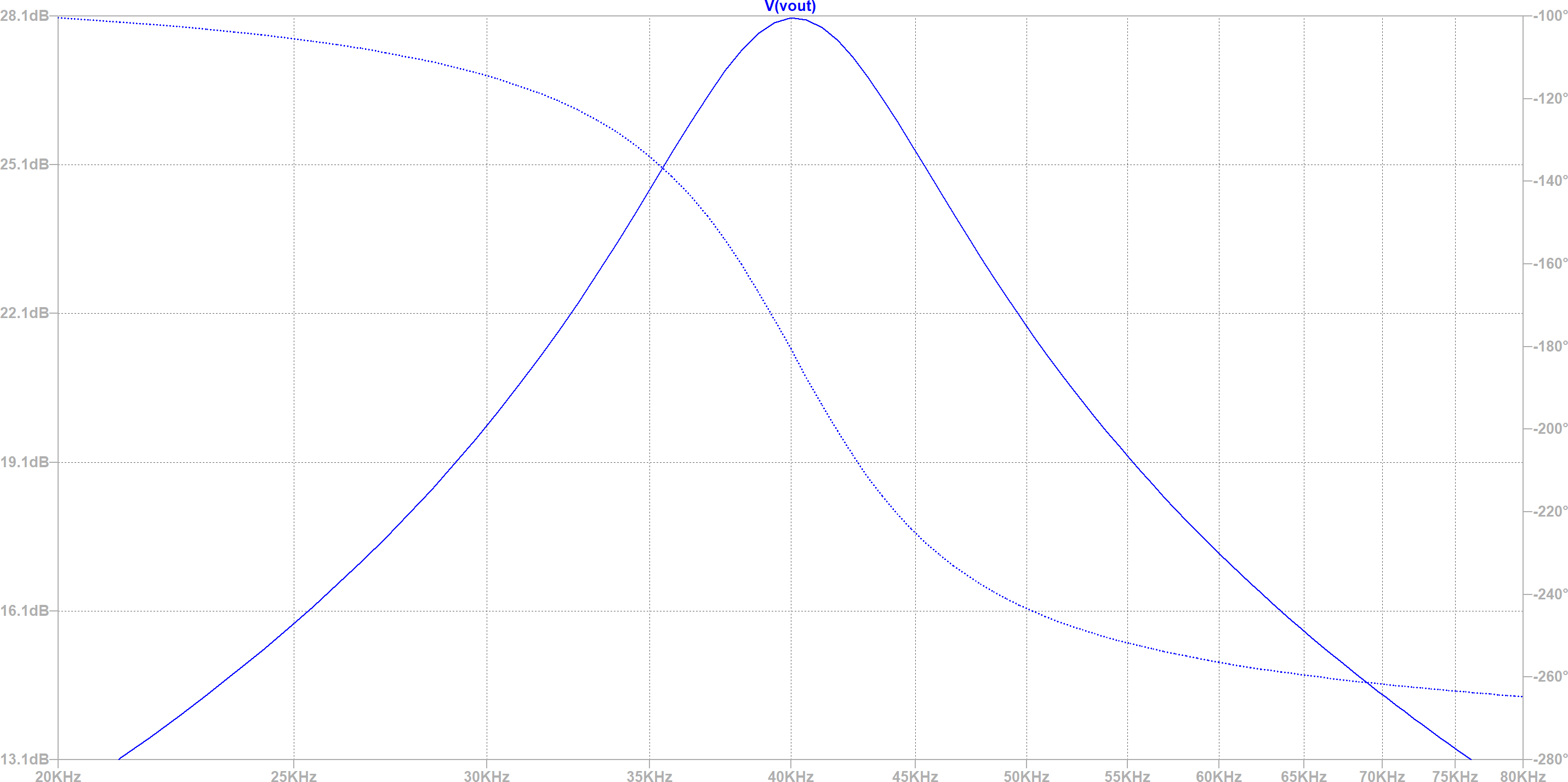
Some time ago, for this project, I designed an active bandpass filter. To simplify its design, I used a 10 MHz GBW op-amp. However a lower GBW op-amp is a much better test for the equation taking into account the GBW. A common and low cost op-amp is the LM324, with a GBW of 1.2 MHz. When making PCBa with JLCPCB, not only the LM324 is very cheap, but there is no component fee. The following example filter with a 1.2 MHz GBW LM324 is designed for a 40 kHz center frequency and a 10 kHz bandwidth. Schematic and simulation results are shown below:

The Excel spreadsheet can be downloaded here and the other files in github

Conclusion

The conclusion will be written in a future release. In the meantime, please find instead a beautiful cat.

Appendix: details of the mathematics

The detailed demonstration of theses equations is a bit long, so it is put in this separate page.